< home
Machine Learning Methods in R
November 2020
An almost comprehensive project comparing and analyzing basic machine learning methods, from simple linear regression to support vector machines and random forest, on a moderate-size construction raw materials dataset with 12 continuous inputs and two discrete inputs.
Requirements
Rprogramming languageTidyversepackageCaretpackage- Other libraries specific to different parts of project
- These are specified in individual
RMarkdownfiles
- These are specified in individual
Machine Learning Methods Used
- Simple Linear Regression
- with basis functions
- Regularized Regression with Elastic net
- pair and triplet interactions
- Logistic Regression
- Generalized Linear Regression
- Neural Network
- single hidden layer, regression and classification
- Random Forest
- regression and classification
- Gradient Boosted Tree
- regression and classification
- Support Vector Machines
- regression and classification
- Multivariate Additive Regression Splines (MARS)
- regression and classification
- Partial Least Squares
Code
Exploratory Data Analysis (EDA):
# Some code snippets

# Read in data
data_url <- 'https://raw.githubusercontent.com/jyurko/CS_1675_Fall_2020/master/HW/final_project/cs_1675_final_project_data.csv'

df <- readr::read_csv(data_url, col_names = TRUE)

step_1_df <- df %>% select(xA, xB, x01:x06, response_1)
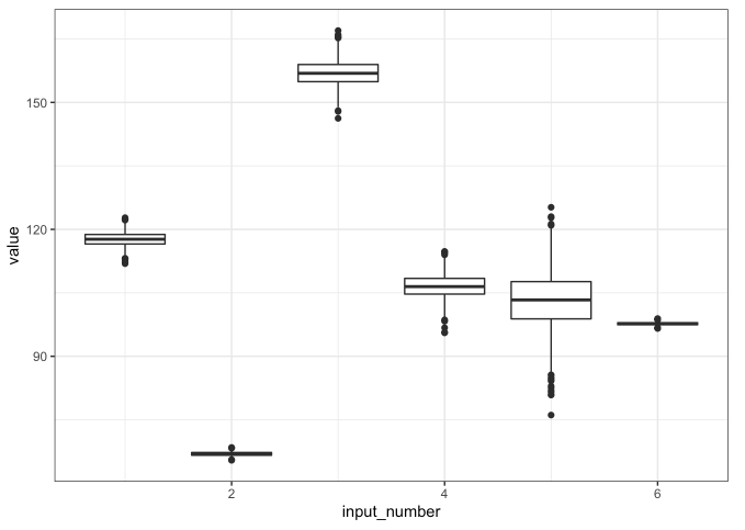
# Variation within variables
## Boxplots
step_1_df %>% tibble::rowid_to_column() %>%
  tidyr::gather(key = "key", value = "value", -rowid, -response_1, -xA, -xB) %>%
  mutate(input_number = as.numeric(stringr::str_extract(key, "\\d+"))) %>%
  ggplot(mapping = aes(x = input_number, y = value)) +
  geom_boxplot(mapping = aes(group = input_number)) +
  theme_bw()
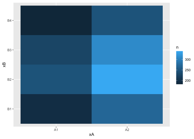
# Covariation between variables
## geom_tile (between categorical inputs)
df %>%
  count(xA, xB) %>%
  ggplot(mapping = aes(x = xA, y = xB)) +
  geom_tile(mapping = aes(fill = n))
Regression Analysis:
# lm() to all inputs
mod_lm_step1 <- lm(response_1 ~ ., step_1_df)
# lm() to a self-devised basis function
mod_lm_basis <- lm(response_1 ~ xA + xB*(splines::ns(x01, df = 2) + splines::ns(x02, df = 2) + splines::ns(x03, df = 2)), step_1_df)
Examine part iiA Examine part iiB Examine part iiB
Binary Classification Analysis:
# Training control settings
my_ctrl <- caret::trainControl(method = "repeatedcv",
                               number = 5,
                               repeats = 5,
                               savePredictions = TRUE,
                               summaryFunction = twoClassSummary,
                               classProbs = TRUE)
roc_metric <- "ROC"
# Logistic regression with additive terms
set.seed(12345)
mod_glm <- caret::train(outcome_2 ~ .,
                            method = "glm",
                            metric = roc_metric,
                            trControl = my_ctrl,
                            preProcess = c("center", "scale"),
                            data = step_2_b_df)

confusionMatrix.train(mod_glm)

# Regularized regression with elastic net
## Custom tuning grid
enet_grid <- expand.grid(alpha = seq(0.1, 0.9, by = 0.1),
                         lambda = exp(seq(-6, 0.5, length.out = 25)))

set.seed(12345)
mod_glmnet_2_b <- caret::train(outcome_2 ~ (.)^2,
                               method = "glmnet",
                               preProcess = c("center", "scale"),
                               tuneGrid = enet_grid,
                               metric = roc_metric,
                               trControl = my_ctrl,
                               data = step_2_b_df)
Examine part iii Examine part iv
Interpretation of Results:
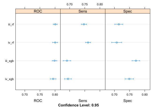
# Evaluating response_1 as a feature
## Area under the ROC curve (AUC)
results <- resamples(list(iii_rf = iii_models$iii_rf,
                          iii_xgb = iii_models$iii_xgb,
                          iv_rf = iv_models$iv_rf,
                          iv_xgb = iv_models$iv_xgb))

dotplot(results)

## Based on AUC, models including response_1 (intermediate input) as feature yield better performance in predicting outcome_2 (output variable); observed from the higher AUC values
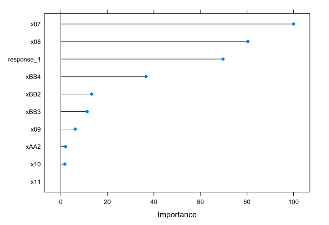
# Variable importance
## Models with response_1 as a feature
plot(varImp(iii_models$iii_rf))